Sparse Filtering in Theano
Sparse Filtering is a form of unsupervised feature learning that learns a sparse representation of the input data without directly modeling it. This algorithm is attractive because it is essentially hyperparameter-free making it much easier to implement relative to other existing algorithms, such as Restricted Boltzman Machines, which have a large number of them. Here I will review a selection of sparse representation models for computer vision as well as Sparse Filtering’s place within that space and then demonstrate an implementation of the algorithm in Theano combined with the L-BFGS method in SciPy’s optimizaiton library.
Sparse Representation Models for Computer Vision
Models employing sparsity-inducing norms are ubiquitous in the statistical modeling of images. Their employment is strongly motivated by the inextricably woven web of a sparse code’s efficiency, functionality, and input distribution match — a rather uncanny alignment of properties. Representing an input signal with a few number of active units has obvious benefits in efficient energy usage; the fewer units that can be used to provide a good representation, without breaking the system, the better. A sparse coding scheme also has logically demonstrable functional advantages over the other possible types (i.e., local and dense codes) in that it has high representational and memory capacites (representatoinal capacity grows exponentially with average activity ratio and short codes do not occupy much memory), fast learning (only a few units have to be updated), good fault tolerance (the failure or death of a unit is not entirely crippling), and controlled interference (many representations can be active simultaneously)(Földiák & Young, 1995). Finally, and perhaps most mysteriously, a sparse code is a good representational scheme because it matches the sparse structure, or non-Gaussianity of natural images (Simoncelli & Olshausen, 2001). That is, images can be represented as a combination of a sparse number of elements. Because a sparse code matches the sparse distribution of natural scenes, this provides a good statistiacal model of the input, which is useful because…
...such models provide the prior probabilities needed in Bayesian inference, or, in general, the prior information that the visual system needs on the environment. These tasks include denoising and completion of missing data. So, sparse coding models are useful for the visual system simply because they provide a better statistical model of the input data.
(Hyvärinen, Hurri, & Hoyer, 2009)
Sparse Coding
In the mid 90s, a seminal article by Olshausen and Field marked the beginning of a proliferation of research in theoretical neuroscience, computer vision, and machine learning more generally. There, they first introduced the computational model of sparse coding (Olshausen & Field, 1996) and demonstrated the ability to learn units with receptive fields strongly resembling those observed in biological vision when trained on natural images. Sparse coding is based on the assumption that an input image can be modeled as a linear combination of sparsely activated representational units :
\begin{equation} {I(x, y)} = \sum_i a_i \phi_i(x, y) \end{equation}
Given this linear generative model of images, the goal of sparse coding is then to find some representational units that can be used to represent an image using a sparse activity coefficient vector (i.e., one that has a leptokurtotic distribution with a large peak around zero and heavy tails as can be seen in the figure below).

The optmization problem for finding such a sparse code can be formalized by minimizing the following cost function:
\begin{equation} E = - {\sum_{x, y} \bigg[ {I(x, y)} - \sum_i a_i \phi_i(x, y) \bigg] ^2} - {\sum_i } S\Big(\frac{a_i} {\sigma}\Big) \end{equation}
where is some non-linear function that penalizes non-sparse activations and is a scaling constant. We can see that this is basically a combination of a reconstruction error and a sparsity cost, what can be referred to as sparse-penalized least-squares reconstruction and can be generally represented by:
\begin{equation} \text{cost = [reconstruction error] + [sparseness]} \end{equation}
More generally, this form of problem falls under the more general class of sparse approximation where a good subset of a dictionary must be found to reconstruct the data:
\begin{equation} \min_{\mathbf{\alpha}\in\mathbb{R}^m} \frac{1}{2} \vert\vert \mathbf{x} - \mathbf{D}\alpha\vert\vert^2_2+\lambda\vert\vert \alpha\vert\vert_1 \end{equation}
However, in this case, is not known and thus makes this an unsupervised learning problem.
Sparse Filtering
Sparse Filtering (Ngiam, Chen, Bhaskar, Koh, & Ng, 2011) is an unsupervised learning technique that does not directly model the data (i.e., it has no reconstruction error term in the cost function). The goal of the algorithm is to learn a dictionary that provides a sparse representation by minimizing the normalized entries in a feature value matrix. For each iteration of the algorithm:
- normalization across rows
- normalization across columns
- Objective function = norm of normalized entries
The remaining portion of this subsection is an excerpt from (Hahn, Lewkowitz, Lacombe Jr, & Barenholtz, 2015):
Let be the feature value matrix to be normalized, summed, and minimized. The components
\begin{equation} f^{(i)}_j \end{equation}
represent the feature value ( row) for the example ( column), where
\begin{equation} f^{(i)}_j=\mathbf{w}_j^T\mathbf{x}^{(i)} \end{equation}
Here, the are the input patches and is the weight matrix. Initially random, the weight matrix is updated iteratively in order to minimize the Objective Function.
In the first step of the optimization scheme,
\begin{equation} \widetilde{\mathbf{f}}_j=\frac{\mathbf{f}_j}{\vert\vert\mathbf{f}_j\vert\vert_2} \end{equation}
Each feature row is treated as a vector, and mapped to the unit ball by dividing by its -norm. This has the effect of giving each feature approximately the same variance.
The second step is to normalize across the columns, which again maps the entries to the unit ball. This makes the rows about equally active, introducing competition between the features and thus removing the need for an orthogonal basis. Sparse filtering prevents degenerate situations in which the same features are always active (Ngiam, Chen, Bhaskar, Koh, & Ng, 2011).
\begin{equation} \hat{\mathbf{f}}^{(i)}=\frac{\widetilde{\mathbf{f}}^{(i)}}{\vert\vert\widetilde{\mathbf{f}}^{(i)}\vert\vert_2} \end{equation}
The normalized features are optimized for sparseness by minimizing the norm. That is, minimize the Objective Function, the sum of the absolute values of all the entries of . For datasets of examples we have the sparse filtering objective:
The sparse filtering objective is minimized using a Limited-memory Broyden–Fletcher–Goldfarb–Shanno (L-BFGS) algorithm, a common iterative method for solving unconstrained nonlinear optimization problems.
Implementation in Theano
Theano is a powerful Python library that allows the user to define and optimize functions that are compiled to machine code for faster run time performance. One of the niceset features of this package is that it performs automatic symbolic differentation. This means we can simply define a model and its cost function and Theano will calculate the gradients for us! This frees the user from analytically deriving the gradients and allows us to explore many different model-cost combinations much more quickly. However, one of the drawbacks of this library is that it does not come prepackaged with more sophisticated optimization algorithms, like L-BFGS. Other Python libraries, such as SciPy’s optimize library do contain these optimization algorithms and here I will show how they can be integrated with Theano to optimize sparse filters with respect to their cost function described above.
First we define a SparseFiter class which performs the normalization scheme formalized above.
 1 import theano
 2 from theano import tensor as t
 3
 4 class SparseFilter(object):
 5
 6     """ Sparse Filtering """
 7
 8     def __init__(self, w, x):
 9
10         """
11         Build a sparse filtering model.
12
13         Parameters:
14         ----------
15         w : ndarray
16             Weight matrix randomly initialized.
17         x : ndarray (symbolic Theano variable)
18             Data for model.
19         """
20
21         # assign inputs to sparse filter
22         self.w = w
23         self.x = x
24
25     def feed_forward(self):
26
27         """ Performs sparse filtering normalization procedure """
28
29         f = t.dot(self.w, self.x.T)               # initial activation values
30         fs = t.sqrt(f ** 2 + 1e-8)              # numerical stability
31         l2fs = t.sqrt(t.sum(fs ** 2, axis=1))   # l2 norm of row
32         nfs = fs / l2fs.dimshuffle(0, 'x')      # normalize rows
33         l2fn = t.sqrt(t.sum(nfs ** 2, axis=0))  # l2 norm of column
34         f_hat = nfs / l2fn.dimshuffle('x', 0)   # normalize columns
35
36         return f_hat
37
38     def get_cost_grads(self):
39
40         """ Returns the cost and flattened gradients for the layer """
41
42         cost = t.sum(t.abs_(self.feed_forward()))
43         grads = t.grad(cost=cost, wrt=self.w).flatten()
44
45         return cost, grads
When this object is called, it is initialized with the passed weights and data variables. It also has a feed_forward method for getting the normalized activation values for as well as a get_cost_grads method that returns the cost (defined above) and the gradients wrt the cost. Note that in this implementation, the gradients are flattened out; this has to do with making Theano compatible with SciPy’s optimization library as will be described next.
Now we need to define a function that, when called, will compile a Theano training function for the SparseFilter based on it’s cost and gradients at each training step as well as a callable function for SciPy’s optimization procedure that does the following steps:
- Reshape the new weights
theta_valueconsistent with how they are initialized in the model and convert to float32 - Assign those reshaped and converted weights to the model’s weights
- Get the cost and the gradients based on the compiled training function
- Convert the weights back to float64 and return
Note that in step #3, the gradients returned are already vectorized based on the get_cost_grads method of the SparseFilter class for compatability with SciPy’s optimization framework. The code for accomplishing this is as follows:
 1 import numpy as np
 2
 3 def training_functions(data, model, weight_dims):
 4
 5     """
 6     Construct training functions for the model.
 7
 8     Parameters:
 9     ----------
10     data : ndarray
11         Training data for unsupervised feature learning.
12
13     Returns:
14     -------
15     train_fn : list
16         Callable training function for L-BFGS.
17     """
18
19     # compile the Theano training function
20     cost, grads = model.get_cost_grads()
21     fn = theano.function(inputs=[], outputs=[cost, grads],
22                          givens={model.x: data}, allow_input_downcast=True)
23
24     def train_fn(theta_value):
25
26         """
27         Creates a shell around training function for L-BFGS optimization
28         algorithm such that weights are reshaped before calling Theano
29         training function and outputs of Theano training function are
30         converted to float64 for SciPy optimization procedure.
31
32         Parameters:
33         ----------
34         theta_value : ndarray
35             Output of SciPy optimization procedure (vectorized).
36
37         Returns:
38         -------
39         c : float64
40             The cost value for the model at a given iteration.
41         g : float64
42             The vectorized gradients of all weights
43         """
44
45         # reshape the theta value for Theano and convert to float32
46         theta_value = np.asarray(theta_value.reshape(weight_dims[0],
47                                                      weight_dims[1]),
48                                  dtype=theano.config.floatX)
49
50         # assign the theta value to weights
51         model.w.set_value(theta_value, borrow=True)
52
53         # get the cost and vectorized grads
54         c, g = fn()
55
56         # convert values to float64 for SciPy
57         c = np.asarray(c, dtype=np.float64)
58         g = np.asarray(g, dtype=np.float64)
59
60         return c, g
61
62     return train_fn
Now that we have the model defined and the training environment, we can build the model and visualize what it learns. First we read in some data and preprocess it by centering the mean at zero and whitening to remove pairwise correlations. Finally we convert the data to float32 for GPU compatability.
1 from scipy.io import loadmat
2 from scipy.cluster.vq import whiten
3
4 data = loadmat("patches.mat")['X'] 		# load in the data
5 data -= data.mean(axis=0)			# center data at mean
6 data = whiten(data)				# whiten the data
7 data = np.float32(data.T)			# convert to float32
Next we define the model variables, including the network architecture (i.e., number of neurons and their weights), the initial weights themselves, and a symbolic variable for the data.
1 from init import init_weights
2
3 weight_dims = (100, 256)       		# network architecture
4 w = init_weights(weight_dims)   		# random weights
5 x = t.fmatrix()                 		# symbolic variable for data
The imported method init_weights simply generates random weights with zero mean and unit variance. In addition, these weights are deemed “shared” variables so that they can be updated across all function that they appear in and are designated as float32 for GPU compatability. With this in place, we can then build the Sparse Filtering model and the training functions for its optimization.
1 model = SparseFilter(w, x)
2 train_fn = training_functions(data, model, weight_dims)
Finally, we can train the model using SciPy’s optimization library.
1 from scipy.optimize import minimize
2
3 weights = minimize(train_fn, model.w.eval().flatten(),
4                    method='L-BFGS-B', jac=True,
5                    options={'maxiter': 100, 'disp': True})
With the maximum number of iterations set at 100, this algorithm converges well under a minute. We can then visualize the representations that it has learned by grabbing the final weights and reshaping them.
1 import visualize
2
3 weights = weights.x.reshape(weight_dims[0], weight_dims[1])
4 visualize.drawplots(weights.T, 'y', 'n', 1)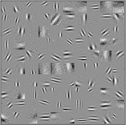
Sparse Filtering Weights
As we can see, Sparse Filtering learns edge-like feature detectors even withough modeling the data directly. Similar outcomes can also be acquired using standard gradient descent methods.
References
- Földiák, P., & Young, M. P. (1995). Sparse coding in the primate cortex. The Handbook of Brain Theory and Neural Networks, 1, 1064–1068.
- Hahn, W. E., Lewkowitz, S., Lacombe Jr, D. C., & Barenholtz, E. (2015). Deep learning human actions from video via sparse filtering and locally competitive algorithms. Multimedia Tools And Applications, 1–14.
- Hyvärinen, A., Hurri, J., & Hoyer, P. O. (2009). Natural Image Statistics: A Probabilistic Approach to Early Computational Vision. (Vol. 39). Springer Science & Business Media.
- Ngiam, J., Chen, Z., Bhaskar, S. A., Koh, P. W., & Ng, A. Y. (2011). Sparse filtering. In Advances in Neural Information Processing Systems (pp. 1125–1133).
- Olshausen, B. A., & Field, D. J. (1996). Emergence of simple-cell receptive field properties by learning a sparse code for natural images. Nature, 381(6583), 607–609.
- Simoncelli, E. P., & Olshausen, B. A. (2001). Natural image statistics and neural representation. Annual Review of Neuroscience, 24(1), 1193–1216.
Posted in Programming with tags: Sparse Filtering, Sparse Coding, Theano, Python