Visualizing CIFAR-10 Categories with WordNet and NetworkX
In this post, I will describe how the object categories from CIFAR-10 can be visualized as a semantic network. CIFAR-10 is a database of images that is used by the computer vision community to benchmark the performance of different learning algorithms. For some of the work that I’m currently working on, I was interested in the semantic relations between the object categories, as other research has been in the past. We can do this by defining their relations with WordNet and then visualizing them using NetworkX combined with Graphviz.
Python Dependencies
Before being able to run the code described in this post, there are a couple of dependencies that must be installed (if not already on your machine). This includes the NetworkX installation, NLTK installation, and Graphviz installation. Also, after installing NLTK, import nltk and use nltk.download() to futher install the wordnet and wordnet_ic databases. You should be all set at this point!
Visualizing CIFAR-10 Semantic Network
For this code demonstration, we do not actually need the CIFAR-10 dataset, but rather its object categories. One alternative would be to download the dataset and use the batches.meta file to import the labels. For simplicity, I instead just list out the categories and put them into a set.
 1 categories = set()
 2 categories.add('airplane')
 3 categories.add('automobile')
 4 categories.add('bird')
 5 categories.add('cat')
 6 categories.add('deer')
 7 categories.add('dog')
 8 categories.add('frog')
 9 categories.add('horse')
10 categories.add('ship')
11 categories.add('truck')
Now we need to define a function that, beginning with a given object class, recursively adds a node and an edge between it and its hypernym all the way up to the highest node (i.e., “entity”). I found this post that demonstrated code that could do this, so I borrowed it and modified it for my purposes. The major addition was to extend the graph building function to mulitple object categories. We define a function wordnet_graph that builds us our network:
 1 import networkx as nx
 2 import matplotlib.pyplot as pl
 3 from nltk.corpus import wordnet as wn
 4
 5 def wordnet_graph(words):
 6
 7     """
 8     Construct a semantic graph and labels for a set of object categories using
 9     WordNet and NetworkX.
10
11     Parameters:
12     ----------
13     words : set
14         Set of words for all the categories.
15
16     Returns:
17     -------
18     graph : graph
19         Graph object containing edges and nodes for the network.
20     labels : dict
21         Dictionary of all synset labels.
22     """
23
24     graph = nx.Graph()
25     labels = {}
26     seen = set()
27
28     def recurse(s):
29
30         """ Recursively move up semantic hierarchy and add nodes / edges """
31
32         if not s in seen:                               # if not seen...
33             seen.add(s)                                 # add to seen
34             graph.add_node(s.name)                      # add node
35             labels[s.name] = s.name().split(".")[0]     # add label
36             hypernyms = s.hypernyms()                   # get hypernyms
37
38             for s1 in hypernyms:                        # for hypernyms
39                 graph.add_node(s1.name)                 # add node
40                 graph.add_edge(s.name, s1.name)         # add edge between
41                 recurse(s1)                             # do so until top
42
43     # build network containing all categories
44     for word in words:                                  # for all categories
45         s = wn.synset(str(word) + str('.n.01'))         # create synset
46         recurse(s)                                      # call recurse
47
48     # return the graph and labels
49     return graph , labels
Now we’re ready to create the graph for visualizing the semantic network for CIFAR-10.
1 # create the graph and labels
2 graph, labels = wordnet_graph(categories)
3
4 # draw the graph
5 nx.draw_graphviz(graph)
6 pos=nx.graphviz_layout(graph)
7 nx.draw_networkx_labels(graph, pos=pos, labels=labels)
8 pl.show()
The resulting semantic network should look like the following:
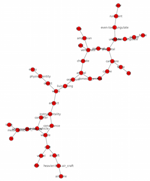
Semantic Network for CIFAR-10
We can see that from entity, the main branch between categories in CIFAR-10 is between artifacts and living things. The object categories themselves tend to be terminal nodes (except for dog).
Quantifying Semantic Similarity
We can also use WordNet to quantify the semantic distance between two given object categories. Developing quantifications for semantic similarity is an area of ongoing study and the NLTK includes a couple variations. Here, we use a simple path_similarity quantification which is the length of the shortest path between two nodes, but many others can be implemented by using the wordnet_ic dataset and defining an information content dictionary (see here).
To find the semantic distance between all object categories, we create an empty similarity matrix of size , where equals the number of object categoes, and iteratively calculate the semantic similarity for all pair-wise comparisons.
 1 import numpy as np
 2 from nltk.corpus import wordnet_ic
 3
 4 # empty similarity matix
 5 N = len(categories)
 6 similarity_matrix = np.zeros((N, N))
 7
 8 # initialize counters
 9 x_index = 0
10 y_index = 0
11 # loop over all pairwise comparisons
12 for category_x in categories:
13     for category_y in categories:
14         x = wn.synset(str(category_x) + str('.n.01'))
15         y = wn.synset(str(category_y) + str('.n.01'))
16         # enter similarity value into the matrix
17         similarity_matrix[x_index, y_index] = x.path_similarity(y)
18         # iterate x counter
19         x_index += 1
20     # reinitialize x counter and iterate y counter
21     x_index = 0
22     y_index += 1
23
24 # convert the main diagonal of the matrix to zeros
25 similarity_matrix = similarity_matrix * abs(np.eye(10) - 1)
We can then visualize this matrix using Pylab. I found this notebook that contained some code for generating a nice comparison matrix. I borrowed that code and only made slight modifications for the current purposes. This code is as follows:
 1 # Plot it out
 2 fig, ax = pl.subplots()
 3 heatmap = ax.pcolor(similarity_matrix, cmap=pl.cm.Blues, alpha=0.8)
 4
 5 # Format
 6 fig = pl.gcf()
 7 fig.set_size_inches(8, 11)
 8
 9 # turn off the frame
10 ax.set_frame_on(False)
11
12 # put the major ticks at the middle of each cell
13 ax.set_yticks(np.arange(similarity_matrix.shape[0]) + 0.5, minor=False)
14 ax.set_xticks(np.arange(similarity_matrix.shape[1]) + 0.5, minor=False)
15
16 # want a more natural, table-like display
17 ax.invert_yaxis()
18 ax.xaxis.tick_top()
19
20 # Set the labels
21
22 # label source:https://en.wikipedia.org/wiki/Basketball_statistics
23 labels = []
24 for category in categories:
25     labels.append(category)
26
27
28 # note I could have used nba_sort.columns but made "labels" instead
29 ax.set_xticklabels(labels, minor=False)
30 ax.set_yticklabels(labels, minor=False)
31
32 # rotate the x-axis labels
33 pl.xticks(rotation=90)
34
35 ax.grid(False)
36
37 # Turn off all the ticks
38 ax = pl.gca()
39 ax.set_aspect('equal', adjustable='box')
40
41 for t in ax.xaxis.get_major_ticks():
42     t.tick1On = False
43     t.tick2On = False
44 for t in ax.yaxis.get_major_ticks():
45     t.tick1On = False
46     t.tick2On = False
This generates the following visualization of the semantic similiary matrix for the CIFAR-10 object categories:
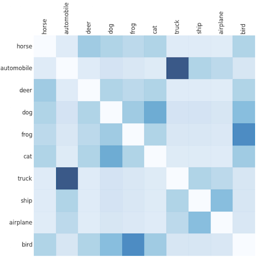
Semantic Similarity Matrix for CIFAR-10 Categories
In this image, bluer colors represent higher similarity (neglecting the main diagonal which was forced to zero for better visualization). As is apparent, all of the object categories belonging to either the artifact or living_thing major branches are closely similar to one another and very different from objects in the opposite branch. Now these semantic distances between object categories can be used for many other types of analyses.
Posted in Programming